The problem at hand is a standard use case for an NLP solution. We have a dataset that consists of many tweets. Some of these tweets pertain to announcing an emergency and some do not. We need to use Natural Language Processing to calssify which is which.
We are given two files. The first one is train.csv which contains the following columns:
- id
- keyword
- location
- text
- target
This file contains about 8,500 tweets that are already classified and need to be used for training our model.
The second file is test.csv which contains the following columns:
- id
- keyword
- location
- text
This file contains 3,700 non-classified tweets which will be used to test the model for it's accuracy.
To solve this problem we need to do the following:
- Import the
train.csvandtest.csvdatasets - Perform text pre-processing such as
- Tokenize the processed data
- Train the model using
train.csv - Test the model using
test.csv
Let us begin by importing the necessary libraries such as NumPy, Pandas, NLTK, Scikit-learn and matplotlib.
1import numpy as np2import pandas as pd34# text processing libraries5import re6import string7import nltk8from nltk.corpus import stopwords910# sklearn11from sklearn import model_selection12from sklearn.feature_extraction.text import TfidfVectorizer13from sklearn.naive_bayes import MultinomialNB1415# matplotlib and seaborn for plotting16import matplotlib.pyplot as plt17import seaborn as sns18from wordcloud import WordCloud1920import random2122nltk.download(['stopwords', 'wordnet'])
1[nltk_data] Downloading package stopwords to /home/karan/nltk_data...2[nltk_data] Package stopwords is already up-to-date!3[nltk_data] Downloading package wordnet to /home/karan/nltk_data...4[nltk_data] Package wordnet is already up-to-date!5678910True
1train_csv = "./data/train.csv"2test_csv = "./data/test.csv"3submission_csv = "./data/submission.csv"
We load the datasets using Pandas
1train = pd.read_csv(train_csv)2print('Training data shape: ', train.shape)3print(train.head())45print()67test = pd.read_csv(test_csv)8print('Testing data shape: ', test.shape)9print(test.head())
1Training data shape: (7613, 5)2 id keyword location text \30 1 NaN NaN Our Deeds are the Reason of this #earthquake M...41 4 NaN NaN Forest fire near La Ronge Sask. Canada52 5 NaN NaN All residents asked to 'shelter in place' are ...63 6 NaN NaN 13,000 people receive #wildfires evacuation or...74 7 NaN NaN Just got sent this photo from Ruby #Alaska as ...89 target100 1111 1122 1133 1144 11516Testing data shape: (3263, 4)17 id keyword location text180 0 NaN NaN Just happened a terrible car crash191 2 NaN NaN Heard about #earthquake is different cities, s...202 3 NaN NaN there is a forest fire at spot pond, geese are...213 9 NaN NaN Apocalypse lighting. #Spokane #wildfires224 11 NaN NaN Typhoon Soudelor kills 28 in China and Taiwan
Now that the datasets are loaded, we need to begin exploring them.
Firstly, we should see how many columns have missing data and assess if any of these columns will be used to train the model. If yes, we need to try our best to fill them. If not, we can leave them as they are.
Let's see how many values are missing in both datasets for every column:
1print("Missing values in training dataset")2print(train.isnull().sum(), end='\n\n')34print("Missing values in testing dataset")5print(test.isnull().sum(), end='\n\n')
1Missing values in training dataset2id 03keyword 614location 25335text 06target 07dtype: int6489Missing values in testing dataset10id 011keyword 2612location 110513text 014dtype: int64
We know for a fact that the text and the target columns will be used for training. Since both these columns do not have missing data, we can proceed. We will consider filling the remaining columns if need be.
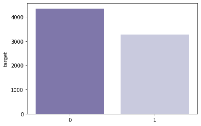
Now, we also need to ensure that there is enough data per class to train the model. For a particular class, if we have too little data to train, we might lose accuracy and if we have too much, we might end up overfitting the data. Since we only have two target values - 0 and 1, let us check the count of both in the training set:
1print(train['target'].value_counts())23sns.barplot(train['target'].value_counts().index,4 train['target'].value_counts(), palette='Purples_r')
10 434221 32713Name: target, dtype: int64456789<matplotlib.axes._subplots.AxesSubplot at 0x7fa0734cb280>
This is a preview of what a disaster and a non-disaster tweet look like:
1# Disaster tweet2disaster_tweets = train[train['target'] == 1]['text']3print(disaster_tweets.values[1])45# Not a disaster tweet6non_disaster_tweets = train[train['target'] == 0]['text']7print(non_disaster_tweets.values[1])
1Forest fire near La Ronge Sask. Canada2I love fruits
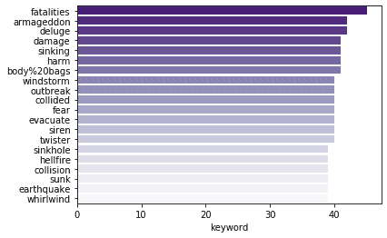
Let us also see what the Top 20 keywords are in order to understand the trend of the tweets
1sns.barplot(y=train['keyword'].value_counts()[:20].index,2 x=train['keyword'].value_counts()[:20], orient='h', palette='Purples_r')
1<matplotlib.axes._subplots.AxesSubplot at 0x7fa070fb6670>
Most of these keywords seem to be related to disasters which means we need to explore further.
Let us now see how many times the word "disaster" has been mentioned in the text and a disaster has actually occured
1train.loc[train['text'].str.contains(2 'disaster', na=False, case=False)].target.value_counts()
11 10220 403Name: target, dtype: int64
As we can see, that's about 71% which is something we need to make a note of.
Let us now explore the "location" column
1train['location'].value_counts()
1USA 1042New York 713United States 504London 455Canada 296 ...7North West London 18Holly Springs, NC 19Ames, Iowa 110( ?å¡ ?? ?å¡), 111London/Bristol/Guildford 112Name: location, Length: 3341, dtype: int64
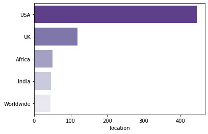
We can see that there are too many unique values. We need to cluster them to understand the trend of this data. For now, we will be brute-forcing this but I am sure that there are better ways to do this.
1# Replacing the ambigious locations name with Standard names2train['location'].replace({'United States': 'USA',3 'New York': 'USA',4 "London": 'UK',5 "Los Angeles, CA": 'USA',6 "Washington, D.C.": 'USA',7 "California": 'USA',8 "Chicago, IL": 'USA',9 "Chicago": 'USA',10 "New York, NY": 'USA',11 "California, USA": 'USA',12 "FLorida": 'USA',13 "Nigeria": 'Africa',14 "Kenya": 'Africa',15 "Everywhere": 'Worldwide',16 "San Francisco": 'USA',17 "Florida": 'USA',18 "United Kingdom": 'UK',19 "Los Angeles": 'USA',20 "Toronto": 'Canada',21 "San Francisco, CA": 'USA',22 "NYC": 'USA',23 "Seattle": 'USA',24 "Earth": 'Worldwide',25 "Ireland": 'UK',26 "London, England": 'UK',27 "New York City": 'USA',28 "Texas": 'USA',29 "London, UK": 'UK',30 "Atlanta, GA": 'USA',31 "Mumbai": "India"}, inplace=True)3233sns.barplot(y=train['location'].value_counts()[:5].index,34 x=train['location'].value_counts()[:5], orient='h', palette='Purples_r')
1<matplotlib.axes._subplots.AxesSubplot at 0x7fa07143c940>
1train['location'].value_counts()
1USA 4452UK 1183Africa 514India 465Worldwide 456 ...7Quito, Ecuador. 18Im Around ... Jersey 19New Brunswick, NJ 110England. 111London/Bristol/Guildford 112Name: location, Length: 3312, dtype: int64
As we can see, the clustering is much better now
Now, we begin exploring the most important column which is the "text" column
1train['text'].head()
10 Our Deeds are the Reason of this #earthquake M...21 Forest fire near La Ronge Sask. Canada32 All residents asked to 'shelter in place' are ...43 13,000 people receive #wildfires evacuation or...54 Just got sent this photo from Ruby #Alaska as ...6Name: text, dtype: object
Before we begin working on our model, we need to clean up the text column. There are a few basic transformations we can do such as making the text lowercase, removing special symbols, removing links and removing words containing numbers like so:
1def clean_text(text):2 text = text.lower()3 text = re.sub('\[.*?\]', '', text)4 text = re.sub('https?://\S+|www\.\S+', '', text)5 text = re.sub('<.*?>+', '', text)6 text = re.sub('[%s]' % re.escape(string.punctuation), '', text)7 text = re.sub('\n', '', text)8 text = re.sub('\w*\d\w*', '', text)9 return text101112# Applying the cleaning function to both test and training datasets13train['text'] = train['text'].apply(lambda x: clean_text(x))14test['text'] = test['text'].apply(lambda x: clean_text(x))1516disaster_tweets = disaster_tweets.apply(lambda x: clean_text(x))17non_disaster_tweets = non_disaster_tweets.apply(lambda x: clean_text(x))1819# Let's take a look at the updated text20print(train['text'].head())21print()22print(test['text'].head())
10 our deeds are the reason of this earthquake ma...21 forest fire near la ronge sask canada32 all residents asked to shelter in place are be...43 people receive wildfires evacuation orders in...54 just got sent this photo from ruby alaska as s...6Name: text, dtype: object780 just happened a terrible car crash91 heard about earthquake is different cities sta...102 there is a forest fire at spot pond geese are ...113 apocalypse lighting spokane wildfires124 typhoon soudelor kills in china and taiwan13Name: text, dtype: object
As we can see, the text looks a lot better now. After this, we break each sentence down to a list of words. This process is called tokenization.
1# Tokenizing the training and the test set2tokenizer = nltk.tokenize.RegexpTokenizer(r'\w+')3train['text'] = train['text'].apply(lambda x: tokenizer.tokenize(x))4test['text'] = test['text'].apply(lambda x: tokenizer.tokenize(x))5train['text'].head()
10 [our, deeds, are, the, reason, of, this, earth...21 [forest, fire, near, la, ronge, sask, canada]32 [all, residents, asked, to, shelter, in, place...43 [people, receive, wildfires, evacuation, order...54 [just, got, sent, this, photo, from, ruby, ala...6Name: text, dtype: object
Next, we remove common structural words from the sentences. These words occur very frequently and help form the sentence. In this case, these stopwords aren't needed.
1def remove_stopwords(text):2 words = [w for w in text if w not in stopwords.words('english')]3 return words456train['text'] = train['text'].apply(lambda x: remove_stopwords(x))7print(train.head())8print()9test['text'] = test['text'].apply(lambda x: remove_stopwords(x))10print(test.head())
1id keyword location text \20 1 NaN NaN [deeds, reason, earthquake, may, allah, forgiv...31 4 NaN NaN [forest, fire, near, la, ronge, sask, canada]42 5 NaN NaN [residents, asked, shelter, place, notified, o...53 6 NaN NaN [people, receive, wildfires, evacuation, order...64 7 NaN NaN [got, sent, photo, ruby, alaska, smoke, wildfi...78 target90 1101 1112 1123 1134 11415 id keyword location text160 0 NaN NaN [happened, terrible, car, crash]171 2 NaN NaN [heard, earthquake, different, cities, stay, s...182 3 NaN NaN [forest, fire, spot, pond, geese, fleeing, acr...193 9 NaN NaN [apocalypse, lighting, spokane, wildfires]204 11 NaN NaN [typhoon, soudelor, kills, china, taiwan]
After removing the stopwords, we should essentially be left with tokenized keywords. We can see the most common words and their promincence by generating a Wordcloud like so:
1def purple_color_func(word, font_size, position, orientation, random_state=None,2 **kwargs):3 return "hsl(270, 50%%, %d%%)" % random.randint(50, 60)456fig, (ax1, ax2) = plt.subplots(1, 2, figsize=[26, 8])7wordcloud1 = WordCloud(background_color='white',8 color_func=purple_color_func,9 random_state=3,10 width=600,11 height=400).generate(" ".join(disaster_tweets))12ax1.imshow(wordcloud1)13ax1.axis('off')14ax1.set_title('Disaster Tweets', fontsize=40)1516wordcloud2 = WordCloud(background_color='white',17 color_func=purple_color_func,18 random_state=3,19 width=600,20 height=400).generate(" ".join(non_disaster_tweets))21ax2.imshow(wordcloud2)22ax2.axis('off')23ax2.set_title('Non Disaster Tweets', fontsize=40)
1Text(0.5, 1.0, 'Non Disaster Tweets')

We will now lemmatize these tokens to bring them to their base dictionary form i.e. the lemma
1def combine_text(list_of_text):2 combined_text = ' '.join(lemmatizer.lemmatize(token)3 for token in list_of_text)4 return combined_text567lemmatizer = nltk.stem.WordNetLemmatizer()89train['text'] = train['text'].apply(lambda x: combine_text(x))10test['text'] = test['text'].apply(lambda x: combine_text(x))1112print(train['text'].head())13print()14print(test['text'].head())
10 deed reason earthquake may allah forgive u21 forest fire near la ronge sask canada32 resident asked shelter place notified officer ...43 people receive wildfire evacuation order calif...54 got sent photo ruby alaska smoke wildfire pour...6Name: text, dtype: object780 happened terrible car crash91 heard earthquake different city stay safe ever...102 forest fire spot pond goose fleeing across str...113 apocalypse lighting spokane wildfire124 typhoon soudelor kill china taiwan13Name: text, dtype: object
Now that we're done with pre-processing the text, we can begin working on our model. Before we do that, we need to transform these words to numerical vectors. These vectors tell us the degree of presence of the words. This presence needs to be measured across documents and the count of the "non-informational" words needs to decreased as well. We will be using TF-IDF to achieve this. We need to vectorize both our train and test datasets to use them in our model like so:
1tfidf = TfidfVectorizer(min_df=2, max_df=0.5, ngram_range=(1, 2))2train_tfidf = tfidf.fit_transform(train['text'])3test_tfidf = tfidf.transform(test["text"])45print(train_tfidf)6print()7print(test_tfidf)
1(0, 5830) 0.42839102724870352 (0, 3630) 0.4428026679238813 (0, 212) 0.38776689384632524 (0, 5829) 0.27469470513610225 (0, 2800) 0.30390783841841426 (0, 7604) 0.325810379034487457 (0, 2328) 0.4428026679238818 (1, 3479) 0.48450407320801719 (1, 3621) 0.382239660893104910 (1, 1381) 0.424605361511986911 (1, 5177) 0.384281118943850512 (1, 6306) 0.3460725853424494513 (1, 3452) 0.2416566526809203814 (1, 3620) 0.3361886095232073415 (2, 3147) 0.265776482588211116 (2, 6724) 0.2356967182241090617 (2, 3062) 0.222777008142381918 (2, 6594) 0.242459555959329719 (2, 7069) 0.4824865717953965620 (2, 8358) 0.604316594455567521 (2, 538) 0.287118415045732722 (2, 7778) 0.2914873309990229623 (3, 3068) 0.442559640087051224 (3, 1335) 0.302790852795807525 (3, 10334) 0.323938049663664126 : :27 (7611, 2826) 0.40147204440218328 (7611, 1810) 0.1402688507157020529 (7611, 9348) 0.184994701292869830 (7611, 4820) 0.1627201419195539231 (7611, 8273) 0.1657526299128345732 (7611, 5498) 0.138248859924952333 (7611, 4746) 0.1273347935520175434 (7611, 7852) 0.1784614628277756735 (7611, 7159) 0.1156742971715851336 (7611, 1427) 0.119779070632172537 (7612, 10335) 0.303243906780195638 (7612, 7547) 0.275592359240969539 (7612, 4437) 0.274170384901298640 (7612, 5255) 0.275592359240969541 (7612, 7545) 0.2701726731951294442 (7612, 11) 0.295596570227284143 (7612, 10) 0.280172639004265344 (7612, 1348) 0.265373819587369945 (7612, 6484) 0.26005731742096146 (7612, 6483) 0.2417395336152289647 (7612, 5254) 0.2458018245887139748 (7612, 6396) 0.1992500942521499349 (7612, 4426) 0.2123445984713403550 (7612, 1335) 0.2163743408975356651 (7612, 10334) 0.23148612760398095253 (0, 9230) 0.610612027245429854 (0, 4170) 0.543399312297706455 (0, 2061) 0.404859211569802756 (0, 1427) 0.409828205940835457 (1, 8823) 0.3751890121805442358 (1, 8026) 0.4465354304846158659 (1, 4270) 0.3665628187563303460 (1, 3094) 0.344250641897037661 (1, 2800) 0.3499670023650775562 (1, 2515) 0.4170668988249362563 (1, 1684) 0.33247677976055764 (2, 8914) 0.298287633973165165 (2, 8739) 0.309665139714840266 (2, 8097) 0.289170066039756267 (2, 7189) 0.3838423385678186368 (2, 3621) 0.302824627167967469 (2, 3620) 0.266341253283638770 (2, 3545) 0.4073857219941351471 (2, 3452) 0.1914494837604612572 (2, 1390) 0.3434929606150824473 (2, 76) 0.317700892923467374 (3, 10334) 0.4582013166970611675 (3, 5406) 0.709975374023601176 (3, 415) 0.534777076600266377 (4, 9747) 0.4290379072928337578 : :79 (3260, 5467) 0.364760189323233380 (3260, 4041) 0.44131184709863781 (3260, 4040) 0.38617273709043482 (3260, 2402) 0.3450644746097996783 (3260, 1618) 0.407128286261537384 (3261, 10225) 0.304765642815767485 (3261, 10222) 0.2405231836894827886 (3261, 6766) 0.308971222023501787 (3261, 6765) 0.304765642815767488 (3261, 5890) 0.3528235225721162489 (3261, 5889) 0.3528235225721162490 (3261, 4890) 0.308971222023501791 (3261, 4889) 0.2514776279128561692 (3261, 4553) 0.308971222023501793 (3261, 4234) 0.304765642815767494 (3261, 4229) 0.2547602507613646695 (3262, 10624) 0.386680759564743796 (3262, 7078) 0.248263988882840997 (3262, 6220) 0.3340112059256215698 (3262, 6219) 0.3340112059256215699 (3262, 2930) 0.3059323676289684100 (3262, 2917) 0.2146772887900108101 (3262, 1691) 0.3866807595647437102 (3262, 91) 0.3866807595647437103 (3262, 90) 0.3563580209819999
Let us begin training our classifier using the vectors we just generated. We will be using a Naive Bayes classifier to classify the tweets in the training dataset. Then, we will use this model to predict the class of the tweets in the test dataset like so:
1# Fitting a simple Naive Bayes on TFIDF2clf_NB_TFIDF = MultinomialNB()3scores = model_selection.cross_val_score(4 clf_NB_TFIDF, train_tfidf, train["target"], cv=5, scoring="f1")5print(scores)
1[0.57703631 0.58502203 0.62051282 0.60203139 0.74344718]
1clf_NB_TFIDF.fit(train_tfidf, train["target"])
1MultinomialNB(alpha=1.0, class_prior=None, fit_prior=True)
Finally, we can our trained classifier with the tweets from our test set to see how well our classifier is doing. The predictions are stored in the file data/submission.csv.
1df = pd.DataFrame()2predictions = clf_NB_TFIDF.predict(test_tfidf)3df["id"] = test['id']4df["target"] = predictions5print(df)67df.to_csv(submission_csv, index=False)
1id target20 0 131 2 042 3 153 9 164 11 17... ... ...83258 10861 193259 10865 0103260 10868 1113261 10874 1123262 10875 11314[3263 rows x 2 columns]
| id | target | |
|---|---|---|
| 0 | 0 | 1 |
| 1 | 2 | 0 |
| 2 | 3 | 1 |
| 3 | 9 | 1 |
| 4 | 11 | 1 |
| … | … | … |
| 3258 | 10861 | 1 |
| 3259 | 10865 | 0 |
| 3260 | 10868 | 1 |
| 3261 | 10874 | 1 |
| 3262 | 10875 | 1 |
3263 rows × 2 columns


